6.3 EMP_cor_analysis

In multi-omics data analysis, it is common to observe the relationships between features through a correlation coefficient matrix.

Note：
The module EMP_cor_analysis automatically selects the intersection of data without missing values from two project datasets for analysis when calculating correlations.

🏷️Example1：Analysis of the correlation between microbial species annotation data and scale scoring data.

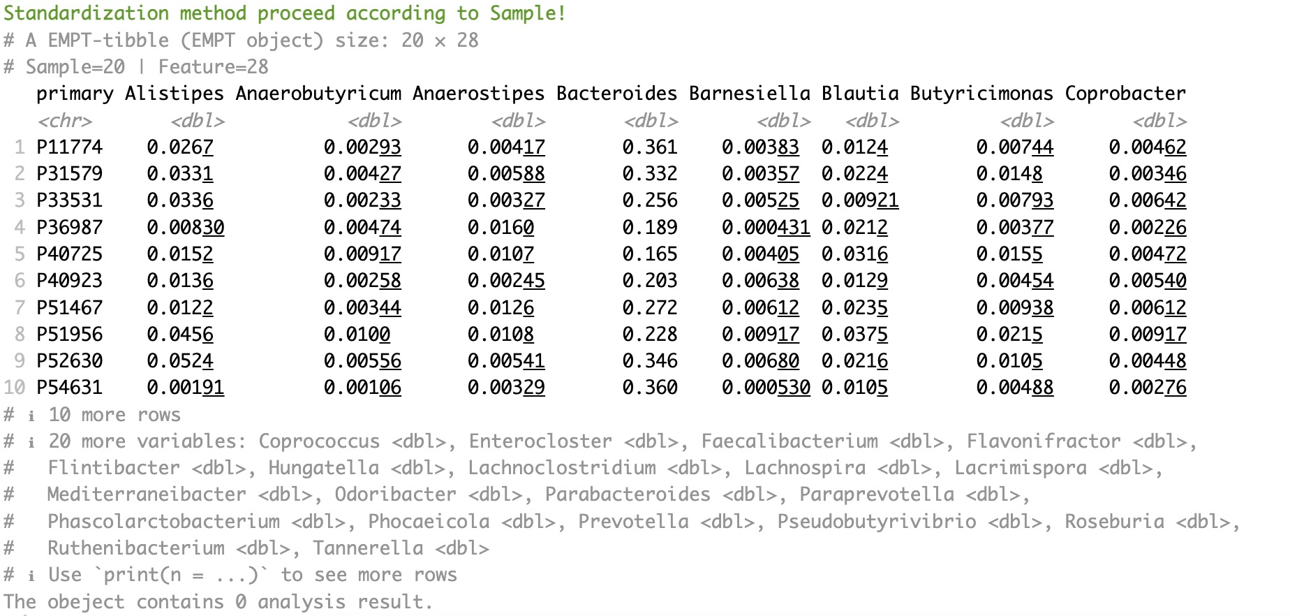
Extract the assay of taxonomy, use module EMP_identify_assay to screen the core data, use module EMP_collapse to collapse out genus-level data, and use module EMP_decostand to standardize relative abundance.

micro_data <- MAE |>
  EMP_assay_extract('taxonomy') |>
  EMP_identify_assay(method='default') |>
  EMP_collapse(estimate_group = 'Genus',collapse_by = 'row') |>
  EMP_decostand(method='relative')
micro_data

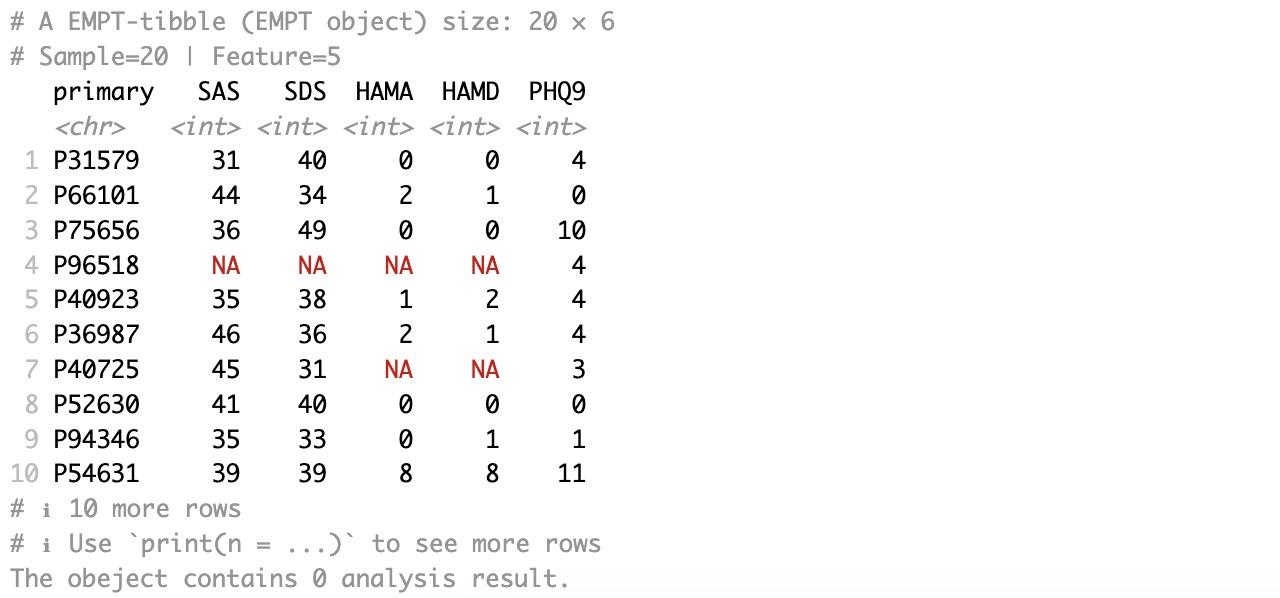
Then, extract the assay of taxonomy from the MAE object, and further extract the scale score data of the corresponding coldata.

meta_data <- MAE |>
  EMP_assay_extract('taxonomy') |>
  EMP_coldata_extract(action = 'add',
                      coldata_to_assay = c('SAS','SDS','HAMA','HAMD','PHQ9','GAD7')) 
meta_data

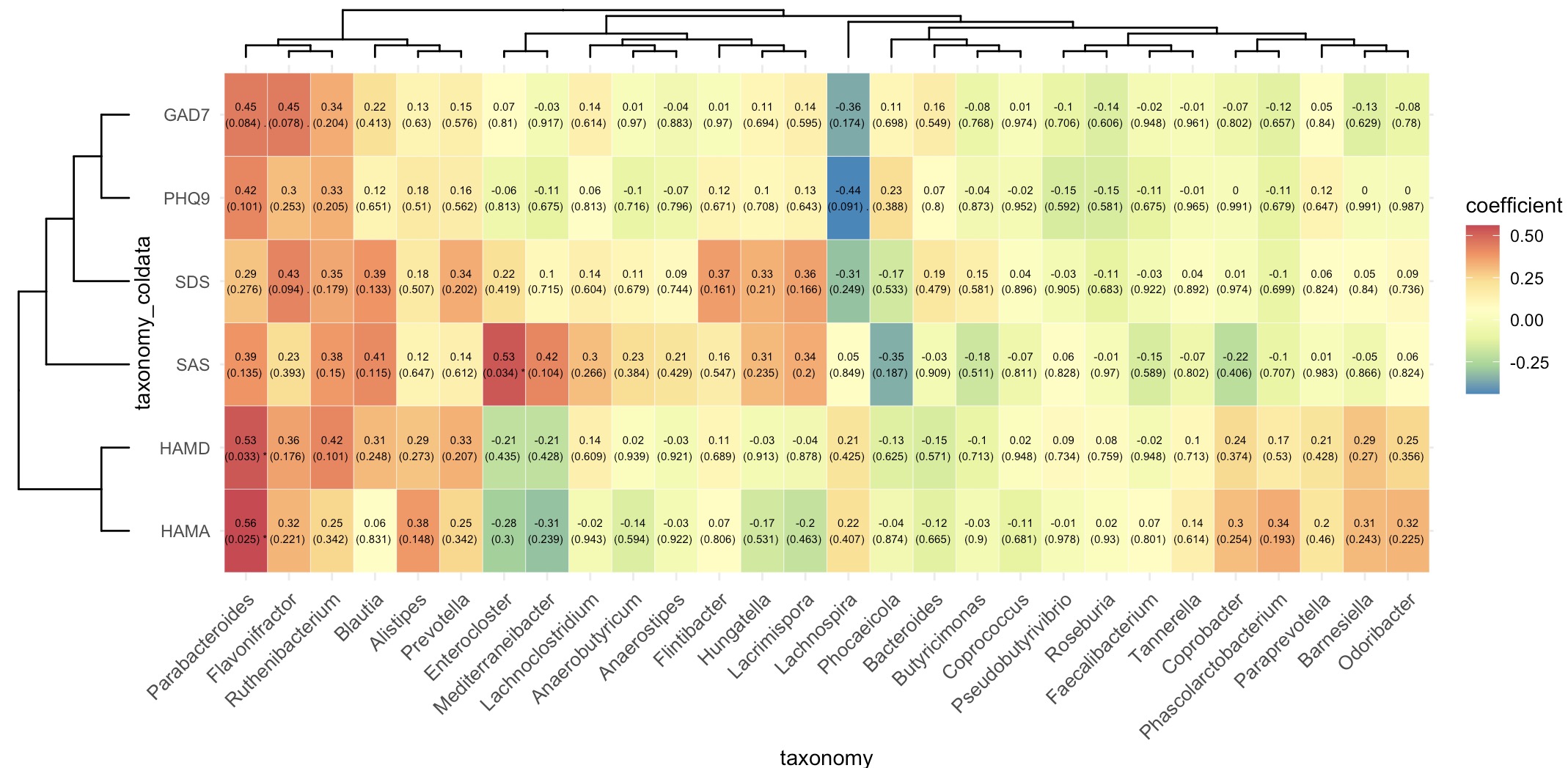
Finally, the microbial abundance data and the scale score data are combined into an EMP object using the + symbol. The correlation analysis and visualization are completed using the modules EMP_cor_analysis and EMP_heatmap_plot.

(micro_data + meta_data) |>
  EMP_cor_analysis() |>
  EMP_heatmap_plot(label_size=2,palette='Spectral',
                   clust_row=TRUE,clust_col=TRUE)

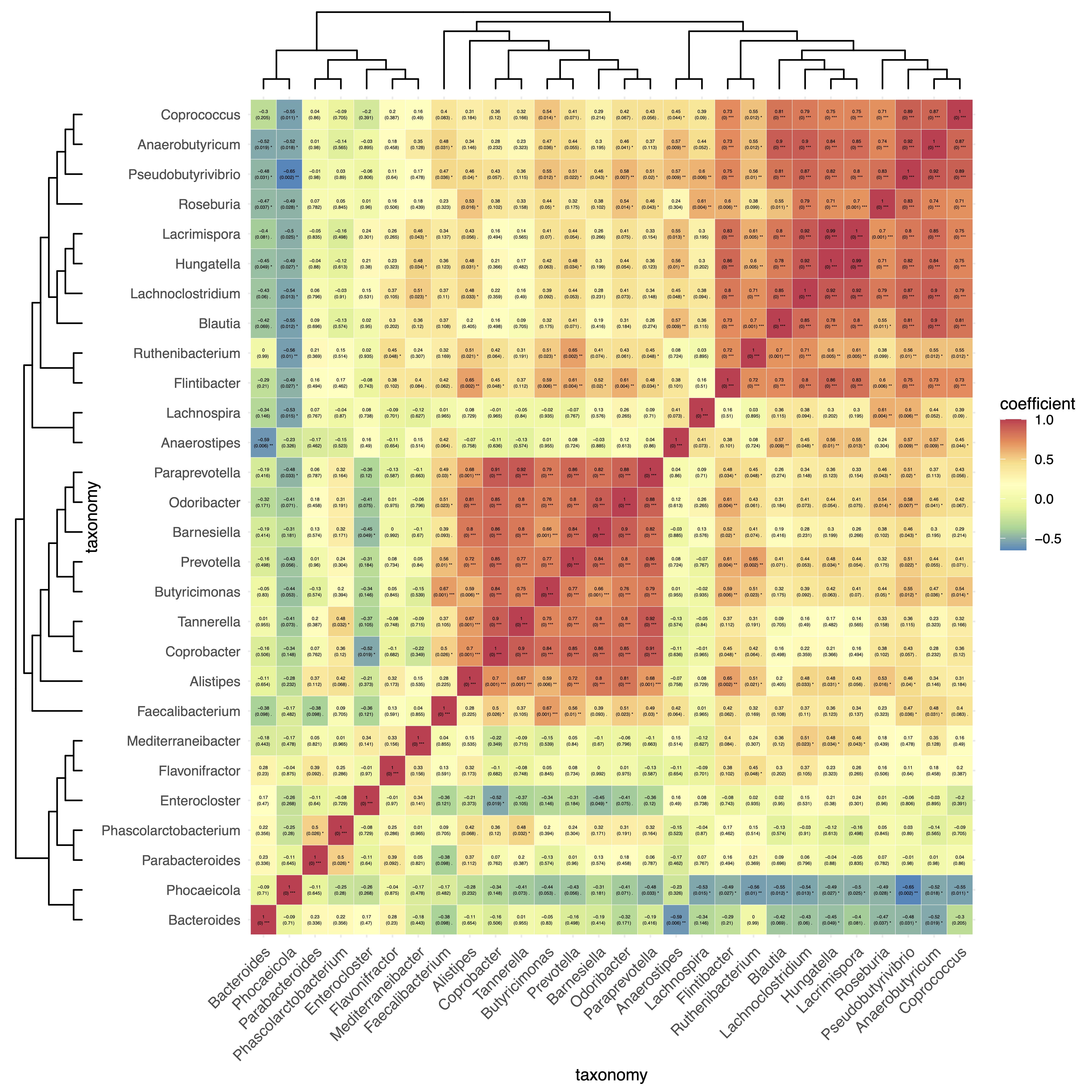
🏷️Example2： Analyse the interrelationships among microbiota.

Note：
① In this example, using NULL here can create an EMP object with only one project.
② When the EMP object contains only one project, autocorrelation calculations will be performed.
③ To draw a co-occurrence network diagram of microbial communities, users can first use the parameter action='get' to obtain the correlation adjacency matrix, and then import it into specialized network analysis tools (such as Cytoscape, MENA, and Gephi) for further analysis.

(micro_data + NULL) |>
  EMP_cor_analysis() |>
  EMP_heatmap_plot(label_size=1,palette='Spectral',clust_row=TRUE,clust_col=TRUE)

6.3.2 Investigate the correlation between differential functional genes of microbiota and differential host genes expression

🏷️Example： Analysis of the correlation between differential functional genes of microbiota and differential host gene expression.

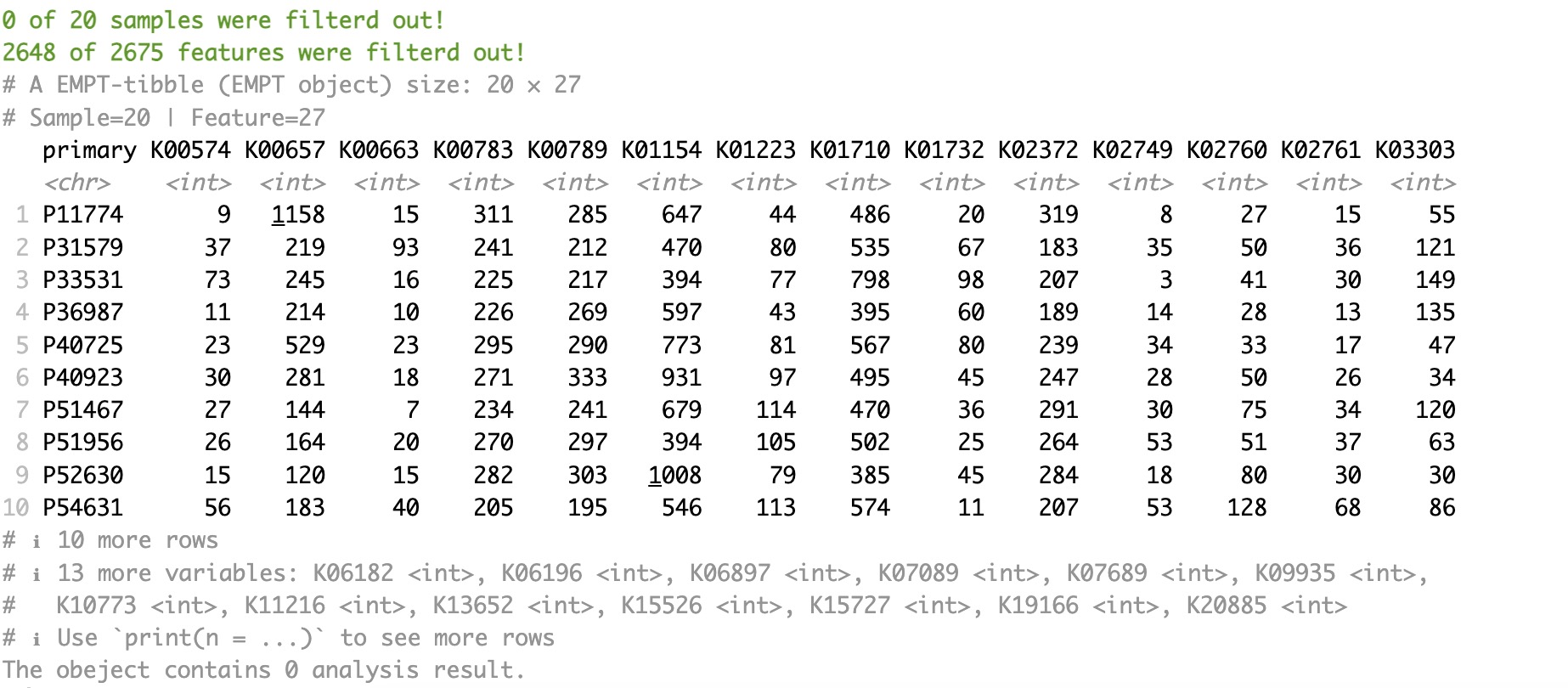
Firstly, extract the assay of geno_ko from the MAE object. Utilize module EMP_identify_assay to filter sparse genes. Apply module EMP_diff_analysis for difference analysis using DESeq2 while accounting for batch issues caused by regional factors. And select KO genes with p-values lower than 0.05.

ko_data <- MAE |>
  EMP_assay_extract('geno_ko') |>
  EMP_identify_assay(method='edgeR') |>
  EMP_diff_analysis(method='DESeq2',.formula = ~Region+Group) |>
  EMP_filter(feature_condition = pvalue < 0.05)
ko_data

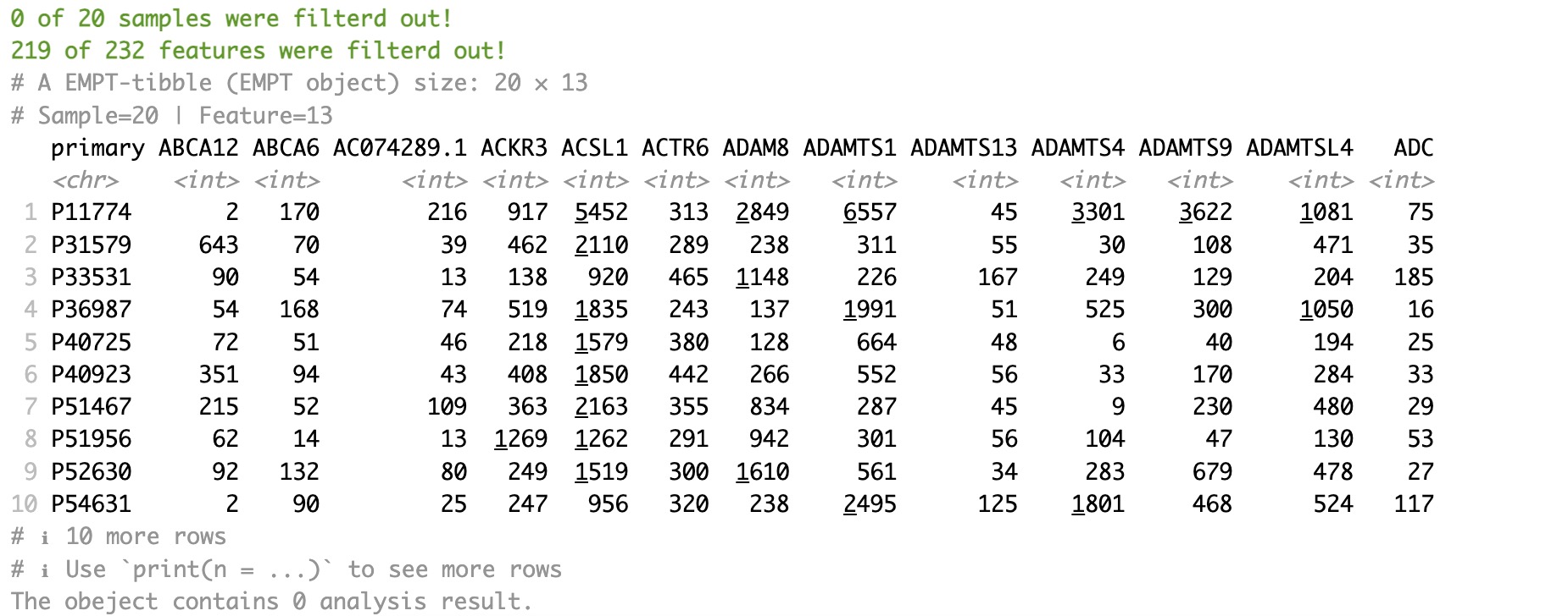
Secondly, extract the assay of host_gene from the MAE object. Utilize module EMP_identify_assay to filter sparse genes. Apply module EMP_diff_analysis for difference analysis using DESeq2 while accounting for batch issues caused by regional factors. And select genes with p-values lower than 0.05.

host_gene <- MAE |>
  EMP_assay_extract('host_gene') |>
  EMP_identify_assay(method='edgeR') |>
  EMP_diff_analysis(method='DESeq2',.formula = ~Region+Group) |>
  EMP_filter(feature_condition = pvalue < 0.05)
host_gene

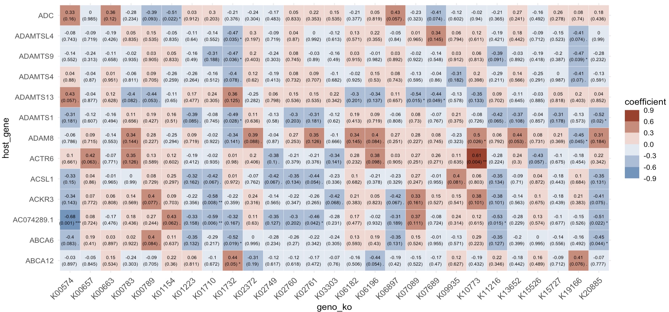
Finally, use the + symbol to merge the ko_data and host_gene into an EMP object. Modules EMP_cor_analysis and EMP_heatmap_plot are utilized to perform correlation analysis and visualization.

(ko_data + host_gene) |>
  EMP_cor_analysis() |>
  EMP_heatmap_plot()

6.3.3 Explore multiple correlations

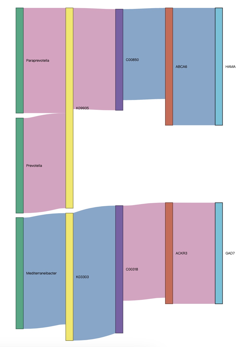
The module EMP_cor_analysis is capable of calculating the interrelationships between multi-omics project datasets. We can separately calculate the distinctive features between individual project datasets, use the + symbol to merge the projects and perform correlation tests in the order of combination. Module EMP_sankey_plot can draw a correlation Sankey diagram based on the results of multiple correlations.

Note：
① In the correlation Sankey diagram, red indicates positive correlation and blue indicates negative correlation.
② The correlation Sankey diagram evaluates the relationships between each node, and isolated nodes will be filtered out.
③ The parameters pvalue and rvalue can adjust the number of edges.

🏷️Example： Explore the multiple correlations between microbial, functional gene, metabolite, host gene, and sample-related data.

micro_data <- MAE |>
  EMP_assay_extract('taxonomy') |>
  EMP_identify_assay(method='default') |>
  EMP_collapse(estimate_group = 'Genus',collapse_by = 'row') |>
  EMP_decostand(method='relative')

ko_data <- MAE |>
  EMP_assay_extract('geno_ko') |>
  EMP_identify_assay(method='edgeR') |>
  EMP_diff_analysis(method='DESeq2',.formula = ~Region+Group) |>
  EMP_filter(feature_condition = pvalue < 0.05)

metabolite_data <- MAE |>
  EMP_assay_extract(experiment = 'untarget_metabol') |>
  EMP_collapse(estimate_group = 'MS2kegg',collapse_by='row',
               na_string = c("NA", "null", "","-"),
               method = 'mean',collapse_sep = '+') |>
  EMP_decostand(method = 'relative') |>
  EMP_dimension_analysis(method = 'pls',estimate_group = 'Group') |>
  EMP_filter(feature_condition = VIP >2)

host_gene <- MAE |>
  EMP_assay_extract('host_gene') |>
  EMP_identify_assay(method='edgeR') |>
  EMP_diff_analysis(method='DESeq2',.formula = ~Region+Group) |>
  EMP_filter(feature_condition = pvalue < 0.05)

meta_data<- MAE |>
  EMP_assay_extract('taxonomy') |>
  EMP_coldata_extract(action = 'add',
                      coldata_to_assay = c('SAS','SDS','HAMA','HAMD','PHQ9','GAD7')) 

(micro_data + ko_data + metabolite_data + host_gene + meta_data) |>
  EMP_cor_analysis() |>
  EMP_sankey_plot()

6.3 EMP_cor_analysis